
Rama is an open source physics simulator for electromagnetic and quantum mechanical systems. It is intended for physics education, and to be an engineering design tool. It simulates two dimensional systems, though it will also simulate some 3D systems that have the right kind of symmetry. Rama is based on the finite element method. Compared to other such simulators, Rama has some unique features:
Rama is fast. Solutions to many interesting problems are produced in a fraction of a second.
Because Rama is fast, it is interactive. You can adjust your model with sliders and see the solution change in real time. This is a good way to develop quick intuitions about many physical situations.
Rama models are created with scripts, rather than with CAD tools. This may seem like a disadvantage, but models created this way can be more easily parameterized and made interactive.
Rama's built in optimization tools quickly solve for optimal configurations.
Rama has many ways to visualize solutions, and can generate all kinds of plots to help you understand your model.
The 2D limitation might seem to rule out using Rama for serious design problems. However there are many 3D problems with symmetries that allow Rama to generate exact solutions, especially problems involving waveguide-fed cavities. Some other problems have 2D models that approximate the full 3D situations, and Rama can provide design intuition in these cases, although not exact solutions. In those cases Rama can often be the starting point for a new design, to get the basics worked out quickly before moving to another simulator's much slower 3D design process.
Rama is available for Mac, Windows and Linux platforms. Here are the installers for the latest stable version:
All Rama development is done on github. If you discover problems please submit an issue here.
Here is an example of interactively changing the width of a horn antenna, to investigate the point at which it starts radiating:
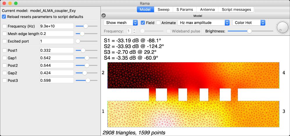
Here we simulate a WR-10 coupler designed for the ALMA radio telescope, to check its performance:
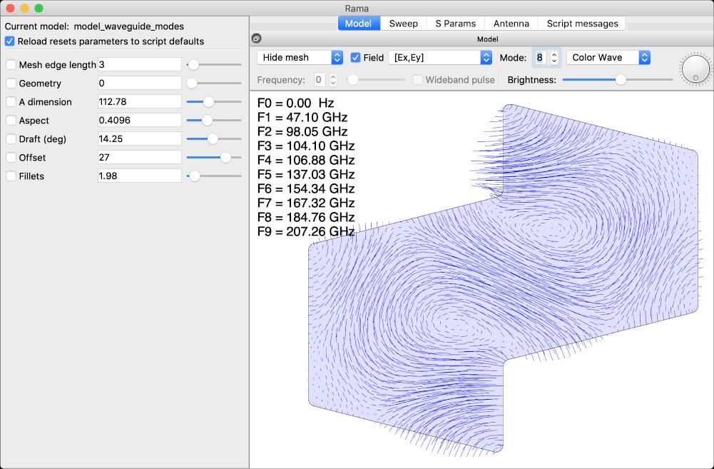
Here we inspect the electric field in a mode of a waveguide:
Here we simulate a quantum mechanical wave packet being deflected by the potential radiating from a point charge.

Rama can solve Maxwell's equations to determine the electromagnetic fields in Ez cavities, which are bounded by walls of constant depth in the Z direction, and where all electric fields point in the Z direction:

The cavity depth is arbitrary, in fact the solution is independent of the depth. A depth of infinity models free space propagation.
The interior of the cavity can be free space or can contain materials with various dielectric properties. The boundary of the cavity can be metal walls, ports (from which energy enters or leaves) or absorbers used in radiation problems. The ports are actually rectangular waveguides. It is assumed that the fields at the ports have the \(TE_{10}\) mode. Energy is injected through excited ports and exits through all ports and boundary absorbers.
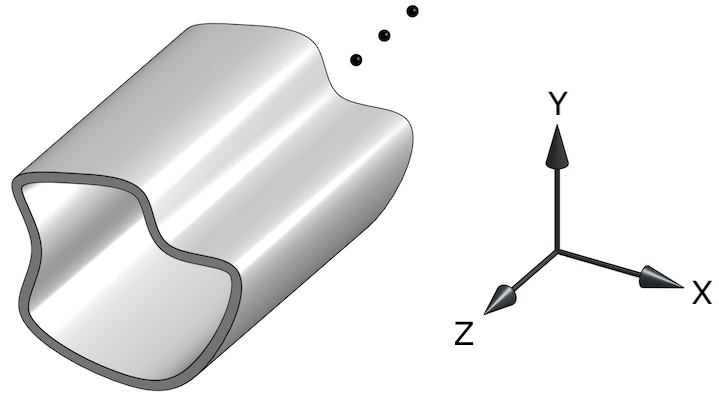
These cavities can be models of real life structures make from sheet metal, or milled out of metal blocks using “split block construction” like so:

Under the hood, Rama computes a 2D field \(\phi(x,y)\) such that the full 3D electric and magnetic phasor fields are
\[\begin{align} \mathbf{E} &= \left[ 0, 0, \phi(x,y) \right] \\ \mathbf{H} &= {i \by \mu \omega} \: \left[ {\del \phi(x,y) \by \del y}, -{\del \phi(x,y) \by \del x}, 0 \right] \end{align}\]where \(\phi\) satisfies the 2D Helmholtz equation with wave number \(k = \omega \sqrt{\mu \epsilon}\).
Rama can solve Maxwell's equations to determine the electromagnetic fields in Exy cavities, which are bounded by walls of constant depth in the Z direction, and where all electric fields are in the XY plane:
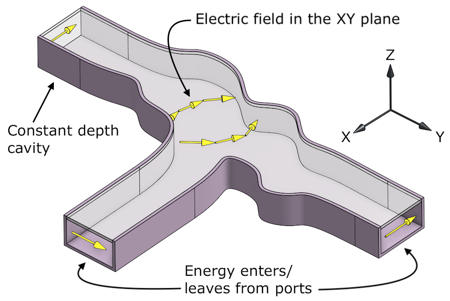
The cavity depth is arbitrary. The solution depends on depth, and if the depth is too small the cavity will not support propagating waves. A depth of infinity models free space propagation.
As with Ez cavities, the interior can be free space or can contain dielectrics, and the boundary can be metal, \(TE_{10}\) ports, or absorbers.
Under the hood, Rama computes a 2D field \(\phi(x,y)\) such that the full 3D electric and magnetic phasor fields are
\[\begin{align} \mathbf{E} &= \alpha {i d \mu \omega \by \pi} \: \cos\left({\pi z \by d}\right) \: \left[ {\del \phi(x,y) \by \del y}, -{\del \phi(x,y) \by \del x}, 0 \right] \\ \mathbf{H} &= \left[ \alpha \: \sin\left({\pi z \by d}\right) {\del \phi(x,y) \by \del x}, \alpha \: \sin\left({\pi z \by d}\right) {\del \phi(x,y) \by \del y}, \cos\left({\pi z \by d}\right) \phi(x,y) \right] \\ \alpha &= { \pi d \by \pi^2-d^2 k_0^2} \end{align}\]where \(d\) is the depth of the cavity and \(\phi\) satisfies the 2D Helmholtz equation with wave number \(k = \sqrt{\omega^2 \mu \epsilon - \pi^2/d^2}\).
Rama can solve for the electric field in ES cavities, which are static or quasi-static situations where the frequency is very low and where all electric fields are in the XY plane. This is a special case of Maxwell's equations. The solution is independent of cavity depth. The interior of the cavity can be free space or can contain dielectrics. The boundaries of the cavity are (by default) dielectrics with \(\epsilon \rightarrow \infty\), or metal containing specified amounts of charge can also be specified.
Under the hood, Rama computes a 2D field \(\phi(x,y)\) such that the full 3D electric field is
\[\begin{align} \mathbf{E} &= \left[ {\del \phi(x,y) \by \del x}, {\del \phi(x,y) \by \del y}, 0 \right] \end{align}\]and the magnetic field is zero. \(\phi\) satisfies Poisson's equation, \(\nabla^2 \phi = \rho / \epsilon\).
Rama can solve Maxwell's equations to determine the electromagnetic fields in waveguides of constant cross section:
The TE and TM modes can be separately computed.
Rama can solve the Schrödinger's equation for nonrelativistic particles in a 2D cavity. The constant frequency (i.e. fixed momentum) Schrödinger equation is solved:
\[\begin{align} \nabla^2 \psi + {2 m \by \hbar} \left( \omega - {V \by \hbar} \right) \psi &= 0 \end{align}\]We use Planck units with \(\hbar=1\) and \(m=1/2\), giving
\[\begin{align} \nabla^2 \psi + ( \omega - V ) \: \psi &= 0 \end{align}\]The wave function \(\psi\) is computed within the cavity. The interior of the cavity can be free space (\(V=0\)) or can contain areas with nonzero \(V\) (in much the same way that electromagnetic cavities can contain dielectric materials).
The boundary of the cavity can be walls where \(\psi=0\), ports (from which waves enter or leave) or absorbers used in radiation problems. The ports behave similarly to those in Ez cavities.
Non constant momentum solutions can be computed using the multi-frequency feature. This allows the behavior of compact wave packets to be studied.
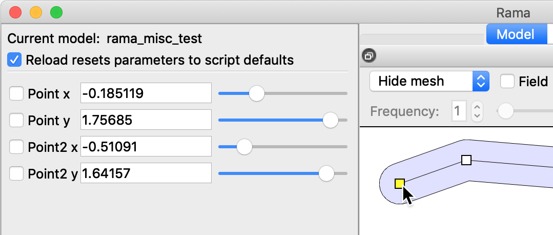
Rama simulations are managed from a single window:

The left hand pane contains the parameters defined by the model, which can be adjusted by entering numerical values or by moving sliders.
The right hand pane contains various tabs that show different aspects of the model. The window under each of these tabs can be dragged away to a separate window - in this way it is possible to see several of those windows at once.
The “model” tab shows the geometry of the model, the mesh, and the field solution.
The “Sweep” tab is a plot that shows values computed as a parameter varies. It is often used to show S-parameters of model ports, but can also plot any user value generated by the script.
The “S Params” tab is a plot that shows S parameters over frequency, for multi-frequency solves.
The “Antenna” tab is a plot that shows the radiation emitted by the model for each angle. It is only useful for models that have radiation boundaries defined.
The “Script messages” tab shows errors and other printed output from the model. When there is a model script error the view will automatically switch to this tab, where the error messages are.
Mouse buttons can be used to change the view in the model tab:
Right click + drag: pan the view.
Mouse wheel: zoom in or out, centered around the mouse pointer.
Control + right click + drag: zoom around the mouse pointer.
Middle click + drag: rotate the view (in 3D mode).
The next two actions are convenient to use on track pads without buttons. For these actions the left button can be held down while dragging, or it can be tapped (pressed and released) before dragging:
Control + left button tap + drag: pans the view.
Command + left button tap + drag: rotates the view in 3D mode.
On the Mac track pad:
Pinch and zoom: zoom around the mouse pointer.
Two finger swipes: pan the view.
On Windows track pads, two finger swipes can be used to zoom.
Model scripts are loaded with the “File / Open” menu command, or are specified on the command line. The script is executed to create the model. If the “Field” checkbox is ticked, the field solution is then computed and displayed. The script is reexecuted (and the field recomputed) when either:
A parameter is changed through its text box or slider.
The script is edited and saved with an external text editor.
The “File / Reload” menu command is selected.
The multi-choice box that defaults to “Hide mesh” can be used to show the mesh, or to draw the dielectric properties into the model.
If the checkbox “Field” is ticked then the field solution is computed and displayed. If it is not ticked then the model geometry (or mesh) is shown.
If the checkbox “Animate” is ticked, then the field solution is computed and animated, so you can get a sense of how the waves flow.
The multi-choice box that defaults to “amplitude and phase” is used to select how the field solution is displayed. The options (which depend on the cavity type) are:
Ez/Hz amplitude and phase. Display the field solution directly, as the amplitude and phase of the electric or magnetic Z component (or in other words, the real part of the phasor \(\phi\)).
Ez/Hz max amplitude. Display the maximum amplitude of the field solution that is ever reached during animation (or in other words, the amplitude of the phasor).
[Ex,Ey] max amplitude. In Exy cavities display the maximum amplitude of the (Ex,Ey) vector.
H & Jsurf amplitude. In Ez cavities display the maximum amplitude of the (Hx,Hy) vector, which is also proportional to the amplitude of the surface current on the constant-Z walls.
Rotated vector E. In Exy cavities display the (Ex,Ey) vector, rotated by 90 degrees.
Vector Jsurf. In Ez cavities display the surface current vector at the constant-Z walls
Vector E, Jsurf. In Exy cavities display the (Ex,Ey) vector, which is also proportional to the surface current on the constant-Z walls.
Vector H. In Ez cavities display the (Hx,Hy) vector.
Poynting vector. Display the Poynting power flow vector.
For ES cavity display the following options are available:
Voltage. Display the voltage.
Absolute voltage. Display the magnitude of the voltage. This is not so useful since nothing physical is changed when a constant is added to the voltage everywhere.
E magnitude. Display the magnitude of the (Ex,Ey) electric field.
Vector E. Display the (Ex,Ey) vector.
Vector isovoltage. Display contours along which the voltage is constant.
For TE or TM waveguide mode display the following options are available:
Ez or Hz to view the Z component of the field.
Ez amplitude or Hz amplitude to view the absolute value of the Z component of the field.
[Ex,Ey] amplitude or [Hx,Hy] amplitude to view the amplitude of the X,Y component of the field.
[Ex,Ey] to view the (Ex,Ey) vector.
[Hx,Hy] to view the (Hx,Hy) vector.
During animation the phase of the displayed solution is rotated. If a maximum amplitude of some kind is being displayed then the animation shows the real part of the amplitude of the rotating phasor. The animation time dial spins during animation. When not animating, you can click and drag the animation time dial to adjust time.
The color scheme used to render the field can be changed with the color multi-choice box. The intensity of the colors (or the length of displayed vectors) can be changed with the brightness slider.
File
Open model: Open a new model script Lua file and executed it to create a new model.
Reload model: Reload the current model script file, and execute it to recreate the model.
Auto-run model on change: Automatically detect when the model script file changes, and reload it when that happens. This is on by default. This makes it convenient to develop models - just save it in your text editor and immediately see the results.
Export boundary as DXF. Export the model boundary shape (config.cd) as a DXF file, so it can be imported into a CAD program. The coordinates in the DXF are in the config.unit units, but the value of config.unit is not saved in the DXF file. Therefore you must set the units manually or scale the model when importing into a CAD program. The values config.dxf_arc_dist and config.dxf_arc_angle can be set to detect and export boundary arcs, otherwise the DXF will only contain line segments.
Export boundary as x,y list Export the model boundary shape (config.cd) as text file list of coordinates.
Export field as matlab data. Save the mesh and current field solution to a matlab file. The following matrices are saved:
p: Mesh point coordinates.
t: Mesh triangles, indexes into p.
u: Solution complex values, one for each point.
In matlab the solution can be visualized with:
  patch('Vertices',p,'Faces',t,'FaceVertexCData',real(u),...
        'FaceColor','interp','EdgeColor','none'); axis equal
Export plot as matlab data. Export the current sweep plot as a matlab file containing an x coordinate vector and a complex y matrix with columns for each port or channel. In matlab, to reproduce the sweep plot in dB use:
plot(x,20*log10(abs(y)))
Export antenna pattern as matlab data. Compute and export the antenna pattern. The following vectors are saved:
azimuth - the azimuths at which the far field is evaluated (radians).
field - the complex values of the far field at each azimuth.
xcorrection, ycorrection - used for phase center correction, as below.
To plot the beam pattern magnitude in dB:
plot(azimuth,20*log10(abs(field)))
To plot the beam phase, assuming a phase center at cx,cy (in config units):
plot(azimuth,angle(field.*(xcorrection.^cx.*ycorrection.^cy)))
Edit
Copy parameters to clipboard. Set the clipboard to a fragment of Lua code that sets the default_parameters table to the current parameter values. This can be pasted in to the Lua script, as a way of saving the current parameter values.
View
Zoom to extents. Set the view so the entire model is visible.
Zoom in / out. Zoom in to or out from the model, around the current mouse pointer position, in case other methods of zooming (like the mouse scroll wheel) are not available.
Set animation time to 0. The animation time controls the phase of the wave or the position of the wideband pulse. This resets the time to zero, starting the animation from the beginning.
Increase / Decrease animation time. Move the current animation time forwards or backwards by one unit.
Show boundary: Select which features of the boundary are displayed: lines, ports, the interior, or vertices. Vertex derivatives with respect to the first checked parameter can also be displayed, as vectors.
Show grid. Toggle the grid.
Show markers. Show the handles for markers, which are 2D parameter values. The handles can be dragged to adjust those parameters.
Show S parameters. Show the computed S-parameters for all ports in the model.
Antialiasing. Render the model and field more smoothly, using antialiasing. On some platforms this can be slow, and so can be switched off.
3D. Toggle 3D view mode, where the solution, boundary, mesh etc are rendered in 3D.
Switch to model after each solve. When this option is turned on, each time a new field solution is computed the model tab is made visible. Turn this option off to allow other tabs to remain visible.
Solve
Sweep. Plot S-parameters or other values over parameter values. See the section on sweeps.
Select optimizer. Select the numerical technique that will be used to perform optimizations. The options are discussed in the section on optimization.
Start optimization. Adjust the selected parameters to improve the output of the config.optimize function. See the section on optimization.
Stop sweep or optimization. Abort the current sweep or optimization, in case it is taking too long.
Run test() after each solve. After each solve, run the config.test function.
Help
Rama manual. Open a web brower at the Rama manual.
Rama website. Open a web brower at the Rama website.
Lua manual. Open a web browser at the Lua manual.
Check for latest version. Check to see if there is a new version of Rama.
Rama can be started from the command line with the following arguments:
filename.lua | The path of a Lua model script file to load and run. |
-unittest | Run all the unit tests, print status and exit. |
-test | Run the config.test() function in the script file then exit. |
-key=value | See the definition of FLAGS in this section. |
Here we design a four port coupler similar to one used in the Atacama Large Millimeter / submillimeter Array (ALMA), a radio telescope. The starting point of the coupler is the paper Designs of Wideband 3dB Branch line Couplers for ALMA Bands 3 to 10.
Physically, the coupler might look like this:

The four ports are rectangular waveguides, with screw holes and pins to support the standard WR-12 waveguide flange connection. The waveguide channels are made with split block construction, i.e. the channels are milled in separate aluminum blocks which are bolted together:

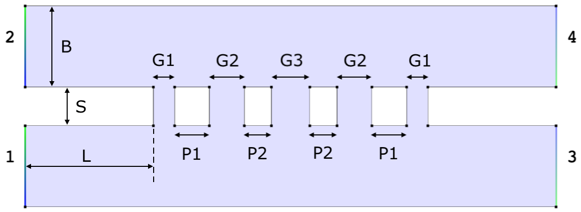
Create a Lua file to model just the active area in the center of the block (the final file is available in the Rama distribution under examples/tutorial_ALMA.lua). This shape will be created:
First add a config table that sets the properties of the simulation. The simulation frequency is set to a parameter so that it is easy to change with a slider:
  config = {
    type = 'Exy',
    unit = 'mm',
    frequency = Parameter{label='Frequency (Hz)', min=75e9, max=115e9, default=93e9},
    mesh_edge_length = 0.2,
    excited_port = 1,
    depth = 2.54,
  }
Then set some variables that will control the geometry. The default values are taken from the above paper:
  -- Basic parameters.
  B = 1.27        -- Waveguide short dimension
  S = 0.605       -- Spacing to other arm of coupler
  L = 2           -- Feed length

  -- Parameters for adjustable post and gap sizes.
  G1 = Parameter{label='Gap 1',  min=0.05, max=1, default=0.332}
  P1 = Parameter{label='Post 1', min=0.05, max=1, default=0.542}
  G2 = Parameter{label='Gap 2',  min=0.05, max=1, default=0.544}
  P2 = Parameter{label='Post 2', min=0.05, max=1, default=0.424}
  G3 = Parameter{label='Gap 3',  min=0.05, max=1, default=0.598}
Now create the geometry itself by adding together rectangles into the shape variable cd:
  -- Create feed-through channels.
  width = 2*L + 2*(G1+P1+G2+P2)+G3
  cd = Rectangle(0, 0, width, B) + Rectangle(0, B+S, width, 2*B+S)

  -- Create the air gaps between the channels.
  x = L
  cd = cd + Rectangle(x, 0, x + G1, 2*B+S)  x = x + G1 + P1
  cd = cd + Rectangle(x, 0, x + G2, 2*B+S)  x = x + G2 + P2
  cd = cd + Rectangle(x, 0, x + G3, 2*B+S)  x = x + G3 + P2
  cd = cd + Rectangle(x, 0, x + G2, 2*B+S)  x = x + G2 + P1
  cd = cd + Rectangle(x, 0, x + G1, 2*B+S)
The ports are specified by selecting points in the middle of each port segment:
  -- Add the ports.
  cd:Port(cd:Select(0, B/2), 1)
  cd:Port(cd:Select(0, S+B*1.5), 2)
  cd:Port(cd:Select(width, B/2), 3)
  cd:Port(cd:Select(width, S+B*1.5), 4)
Finally set the config.cd variable to cd (alternatively config.cd could have been used directly instead of cd above):
config.cd = cd
Running Rama on this file and selecting “Hz max amplitude” to show the amplitude of the waves gives:
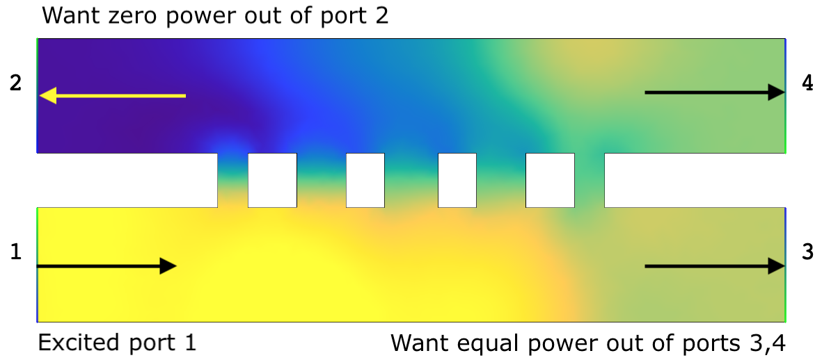
For the coupler to work, power injected on port 1 needs to be equally split between ports 3 and 4, with no power being returned on ports 1 or 2. The displayed S parameters show that the configuration is close to this situation, but is not perfect. To automatically optimize a better configuration, add an optimize function to the config table like so:
  config = {
    ...
    optimize = function(port_power, port_phase, field)
      return port_power[1],                 -- Minimal return loss
             port_power[2],                 -- Minimal output to port 2
             port_power[3] - port_power[4]  -- Balance ports 3 and 4
    end,
  }
The three values returned by optimize will, if they go to zero, result in the desired constraints being achieved. Now tick all gap and post parameters, and run “Solve / Start optimization”. After optimization has finished the situation has improved, particularly the balance of power between ports 3 and 4.
Run “Solve / Sweep” to plot the S-parameters over frequency:

Notice that at the default frequency (93 GHz) ports 3 and 4 are well balanced, but at other frequencies the balance is not so good. To improve this, optimize over multiple frequencies simultaneously. Change config.frequency to be LinearRange(85e9, 100e9, 50), to optimize over 85 GHz to 100 GHz. Now the optimize function needs to be changed to return information for all frequencies:
  optimize = function(port_power, port_phase, field)
    -- Hint to the solver that we're going to be Select()ing all solutions.
    field.SolveAll()
    -- Compute values to optimize over all frequencies.
    local T = {}
    for i = 1,#config.frequency do
      field.Select(i)
      port_power, port_phase = field.Ports()
      table.insert(T, port_power[1])  -- Minimal return loss
      table.insert(T, port_power[2])  -- Minimal output to port 2
      table.insert(T, port_power[3] - port_power[4])  -- Balance ports 3 and 4
    end
    -- Return all values to the optimizer.
    return table.unpack(T)
  end,
After rerunning the optimization, the S-parameters over frequency can be seen using the “S Params” tab:
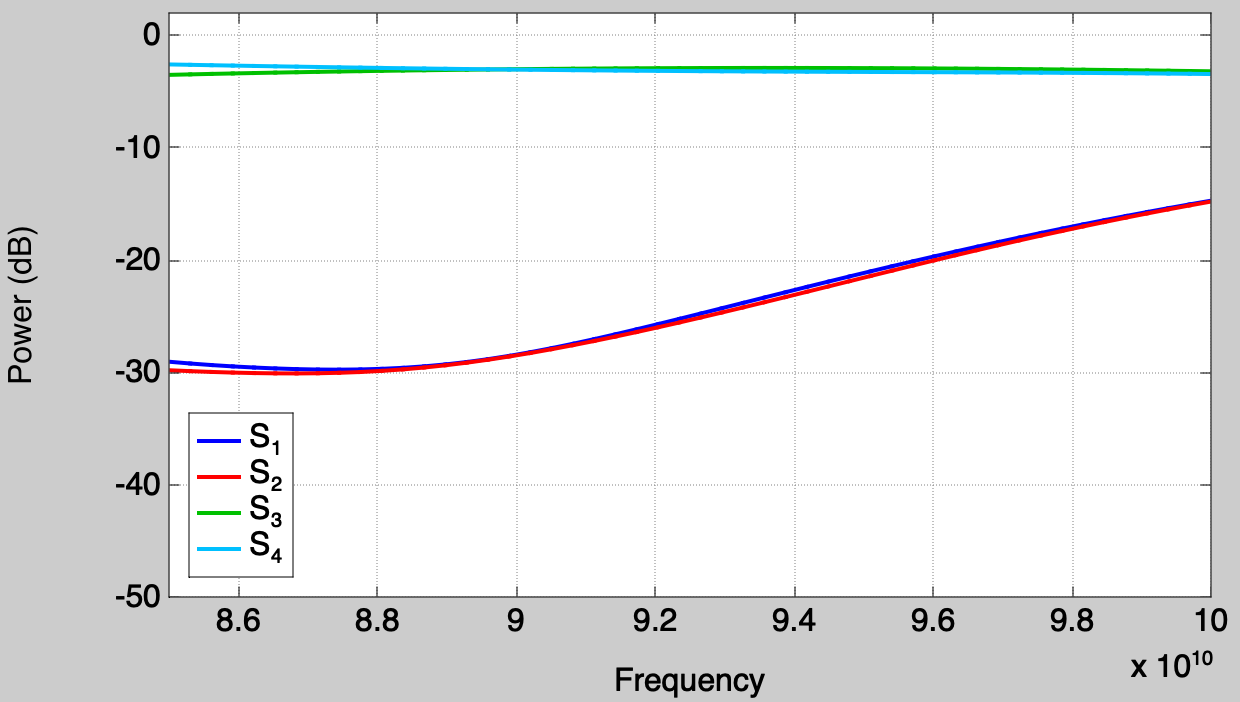
Note that the “Solve / Sweep” command can't be used for this because config.frequency is no longer a single value controlled by a parameter. The balance between ports 3 and 4 is greatly improved across frequency, somewhat at the expense of the power returned on ports 1 and 2. This tradeoff can be adjusted by weighting the values returned by the optimize function.
Simulations in Rama are driven by Lua scripts that specify the boundary of the cavity, the locations of ports, any dielectric materials, and other parameters. Here's the reference manual for Lua, which explains the structure of the language. That has much more detail than you actually need to run Rama, a gentler introduction is the book Programming in Lua. An older version of that book is available online and is still 100% relevant as Rama does not use any advanced Lua features.
The job of the script is to create a Lua table called config that contains the following fields:
type | The type of cavity to simulate: 'S', 'Exy', 'Ez', 'ES', 'TE' or 'TM'. |
unit | The distance unit to use for all geometry numbers. Options are 'nm', 'micron', 'mm', 'cm', 'm', 'km', 'mil' and 'thou' (both mean 0.001 inch), 'inch', 'foot', 'yard', 'mile'. |
cd | The geometry of the “computational domain”. This is a shape object that specifies the boundary polygon, dielectric regions, and the location of ports. Usually most of the script is concerned with creating this object (see the section on shape objects). |
frequency | The frequency in Hz to run the simulation at. This is a single number for a single frequency simulation. For a multi-frequency simulation this is an array of frequencies. For 'ES' cavities this can be set to 1. |
mesh_edge_length | The maximum edge length of the mesh (in the above units). This should usually be no larger than 1/10 of the wavelength. Smaller numbers here result in finer meshes that will have more accurate solutions but which will take longer to solve. |
excited_port | If this is an integer \(\ge 1\), the port to inject a signal on. If this is an array {\(m_1,\phi_1,m_2,\phi_2,\ldots\)} then \(m_i,\phi_i\) specifies the magnitude (not power) and relative phase (in degrees) of the signal to inject on port \(i\). |
depth (optional) | The depth (in the above units) of Exy cavities. This is not used for the other cavities as their solutions are independent of depth. The depth can be set to Infinity to model free space, with solutions that are independent of Z. |
optimize (optional) | When optimization is performed the optimizer calls this function. It is defined as:
  optimize=function(port_power, port_phase, field)
    ...
    return error1,error2, ...
  end
The arguments are arrays of powers (in Watts) and phases (in radians) for each defined port, and a field table that allows the field solution to be interrogated. The return values are one or more error values. The goal of optimization is to get the errors as close to zero as possible. The field table contains functions that can be called with x,y coordinates to return various field derived quantities:
  field.Select(n)       -- Select field for frequency n (1..#config.frequency)
                        -- All functions below return values for this frequency
  field.SolveAll()      -- A hint that Select will be called for all n.
                        -- This pre-solves the fields in parallel, for speed
  field.Ports()         -- The port_power,port_phase for the selected field
  field.Complex(x,y)    -- field components as a complex number
  field.Magnitude(x,y)  -- magnitude of the field
  field.Phase(x,y)      -- phase of the field (in radians)
  field.Poynting(x,y)   -- x,y components of Poynting vector (2 return values)
  field.Power(x,y)      -- magnitude of the Poynting vector
  field.Pattern(theta)  -- antenna power (in W) at angle theta (in degrees)
  field.Directivity()   -- antenna directivity (max power / avg power)
If the returned error or its derivatives are infinity or NaN (i.e. undefined) for the current parameters then the optimizer will not step into this region. If this happens too many times then the optimizer will give up and return a sub optimal result. This can happen in various ways, including
If config.optimize is defined it is also called once for each regular (non optimization) run of the script, to help verify the function contains no runtime errors. For these calls the field functions may return all zeros. |
test (optional) | When the “Run test() after each solve” checkbox is ticked, the test function is called every time a new solution is created. It has exactly the same arguments as optimize:
  test=function(port_power, port_phase, field)
    ...
    return value1,value2,...
  end
The test function can optionally return values, that can be plotted during a sweep. It can also send output to the script messages tab using either print or error. This function is callable when parameters are changed, during sweeps, and optimizations. The test feature can be used to generate reports, and it is also used as part of the internal Rama unit test system. |
antenna_pattern (optional) | For antenna simulations, the way in which the far field antenna pattern will be computed. Options are
|
boresight (optional) | For antenna simulations, the angle that is nominally the highest gain part of the beam. This angle becomes the zero azimuth on the antenna pattern plot. This angle is in degrees, 0 is towards the right and 90 is up. If this is not specified it defaults to 0. |
max_modes | For TE and TM type, this is the number of modes to compute. |
wideband_window (optional) | For a multi-frequency simulation this is the scaling window that is used to display wideband pulses. Valid values are rectangle and hamming. If this field is missing then a rectangular window is assumed. |
dxf_arc_dist (optional) | For DXF export, concentric points closer than this distance to their neighbors are potentially considered to be part of arcs. |
dxf_arc_angle (optional) | For DXF export, concentric points with angles less than this to their neighbors are potentially considered to be part of arcs (degrees). |
The geometry and other parameters of most models will be driven by parameters. Parameters are numerical values that the user can easily adjust via text boxes and sliders in a panel on the user interface.
Parameters are easy to use from within the script. For each parameter you want, call the Parameter() function like this:
value = Parameter{label='Some text', min=0, max=3, default=1}
The label is displayed next to the parameter's text box and slider. Each parameter must have a different label. The bounds of the parameter, i.e. its minimum and maximum value are specified in min and max. The initial value of the parameter is specified by default (which must be between min and max). The returned value of the Parameter() function is the current value of the parameter. The first time the script is run this will be the default, but when the user changes the parameter the script will be rerun, Parameter() will return the new value and an updated solution will be computed for any new geometry.
By default, parameters can take any real value. Parameters that are restricted to integers can be generated by:
  count = Parameter{label='Count', min=1, max=10, default=1,
                    integer=true}
If you have many parameters it can be useful to put them into groups. A horizontal line to separate groups can be generated by calling ParameterDivider().
Parameter values can be used to control shapes or any other aspect of the simulation. For example it is common to use parameters in the config table to allow configuration values to be controlled, like this:
  config = {
    frequency = Parameter{label='Frequency (Hz)', min=10e9,
                          max=20e9, default=15e9},
    excited_port = Parameter{label='Excited port', min=1, max=4,
                             default=1, integer=true},
    ...
  }
If the “Reload resets parameters to script defaults” checkbox is checked then parameters are reset to their default values each time the script is loaded from the filesystem. If it's not checked then parameters keep their current values (actually they take the value of whatever parameter last had the same label, even if the parameter order changed, as long as the min and max values are consistent).
Parameter defaults can come from a variety of places. The rules used to determine the default are:
If the default argument to the Parameter{} function is present, use that number as the default, otherwise:
If the defaults argument is a table then look up the default in that table using the parameter label as a key, otherwise:
If the global default_parameters table exists then look up the default in that table using the parameter label as a key, otherwise:
Use the min value as the default.
Reading defaults from tables allows easy copying of the current parameter values back into the script: simply select “Edit / Copy” from the menu and the current parameters will be copied to the clipboard in this form:
  default_parameters = {
    ['Point x'] = 0.12,
    ['Point y'] = 0.54,
    ...
  }
This block of text can be pasted back into the script so that parameters can acquire their defaults from it.
It is common to have parameters that are actually the x,y coordinates of some point within a shape. Such parameters pairs can be generated automatically and controlled by clicking and dragging on-screen markers, as shown here:
To create a marker you call the ParameterMarker{} function like this:
  x,y = ParameterMarker{label='Point', min={-1,-1}, max={2,2},
                        default={0.5,0.5}}
The min, max and default arguments are similar to Parameter{} except that a table of x,y coordinates is given instead of a number. The label is suffixed with “x” and “y” to create two new parameters. Those parameters can be adjusted by text box, slider, or by clicking and dragging the marker. ParameterMarker{} returns both the x and y parameters values. Note that Lua allows those values to be passed directly as two arguments of another function, so for example the following is a convenient idiom:
shape:AddPoint(ParameterMarker{...})
The following Lua standard libraries can be used: base, table, string, utf8, math, and the time related functions in the os library. The standard Lua print() function sends text to the “script messages” tab. The standard Lua error() function will output its error message to this tab also. The following extra miscellaneous functions are defined:
Draw(s) | For debugging, draw the shape s to the simulation window. The shape will not be simulated. This can be used (for example) to check intermediate stages of shape creation. |
DrawText(x,y, | For debugging, draw the string s at x,y in the simulation window. The optional ha argument is the horizontal alignment of the text which can be 'center', 'right' or the default 'left'. The optional va argument is the vertical alignment of the text which can be 'top', 'bottom', 'center' or the default 'baseline'. |
math.log10(x) | The standard \(\log_{10}\) function, an addition to the math library because it is not defined by Lua. It is useful for computing things in decibels. |
In addition to the standard Lua global variables, the following are available:
FLAGS | A table populated with any -key=value arguments given on the command line. This is useful for testing. For example if -test_number=5 is given on the command line then FLAGS.test_number will return the value '5' (note that this is the string '5' and not the number 5). |
Rama Lua supports vectors in addition to real numbers. Vectors are arrays of numbers that are treated as a single block by math operators. Vector are mostly used by dielectric callback functions, for efficiency reasons. Below are the operations and functions available for vectors (a and b are vectors of the same size and k is a real number).
a + b, a - b, | The elementwise sum (product, etc) of a and b. This result is a vector of the same size as a or b. |
a + k, k + a, etc. | The elementwise sum of a and k. This result is a vector of the same size as a (and likewise for the other operators). |
Vector() | Create a new zero size vector. |
#a | The number of elements in a. |
a.length | The length of a (i.e. its \(L_2\) norm). |
a.normalized | The vector a normalized to unit length. |
a:Resize(n) | Resize the vector to have n elements. All elements will be set to zero. Return a, so that v = Vector():Resize(n) can be written. |
a[i] | Access the i'th element of a, where i is in the range 1...#a. |
a:dot(b) | Return the dot product of a and b. |
a:cross(b) | Return the cross product of 3-vectors a and b. Or, if a and b are 2-vectors, return the Z value of the cross product of two vectors in the XY plane. |
vec.New(a1, a2, ...) | Create a new vector with elements initialized to a1, a2, etc. |
vec.abs(a), vec.acos(a), | Math functions on vectors, similar to the regular functions in the Lua math library. The atan function accepts one argument or two as in Lua 5.3, the atan2 function accepts two arguments as in Lua 5.0. |
vec.eq(a,b) | A vector with ones where \(a = b\) and zero otherwise. Named comparison functions are used for elementwise comparison instead of overloading the comparison operators, because the latter can only return single booleans. |
vec.ne(a,b) | A vector with ones where \(a \ne b\) and zero otherwise. |
vec.lt(a,b) | A vector with ones where \(a < b\) and zero otherwise. |
vec.gt(a,b) | A vector with ones where \(a > b\) and zero otherwise. |
vec.le(a,b) | A vector with ones where \(a \le b\) and zero otherwise. |
vec.ge(a,b) | A vector with ones where \(a \ge b\) and zero otherwise. |
vec.IsVector(a) | True if a is a vector, false otherwise. |
Rama Lua supports complex numbers in addition to real numbers. The real and imaginary parts of the complex numbers can be either real numbers or vectors. Below are the operations and functions available for complex numbers (a and b are complex numbers, k is a real number and v is a vector).
Complex(re,im) | Create a new complex value from the real and (optionally) imaginary parts, which are either both real numbers or both vectors of the same size. |
a + b, a - b, | The complex sum (product, etc). The values a and b must be compatible in the sense that their real and imaginary parts must either both be real numbers or both be vectors of the same size. |
a + k, k + a, etc. | The sum of complex value a and real number k (and likewise for the other operators). |
a + v, a * v, etc. | The sum (product, etc) of complex value a and vector v, which must be compatible. In binary operations the complex value a must appear before the vector v to ensure v is treated as the real part of a complex vector. Due to the way overloaded operators work in Lua, if v appears first then a will be treated as a vector, which will fail. |
a.abs | The absolute value or magnitude of a. |
a.angle | The angle of a in radians. |
a.re, a.im | The real and imaginary parts of a. |
a.conj | The conjugate of a. |
complex.exp(a) | Math functions on complex numbers or vectors, similar to the regular functions in the Lua math library. |
Complex valued vectors in Rama are a Complex object where the real and imaginary parts are Vector objects (not the reverse, i.e. vectors where each value is complex).
The util table contains a variety of helper functions. All of these are implemented in Lua in the user_script_util.lua source file.
c | The speed of light in m/s. |
epsilon0 | The permittivity of free space, \(\epsilon_0\). |
mu0 | The permeability of free space, \(\mu_0\). |
FAR_FIELD | A special material color, see config.antenna_pattern. |
DistanceScale() | Return the distance scale in “meters per unit”. This is the length in meters of one config.unit unit of distance. |
Lambda0InM() | Return the free space wavelength \(\lambda_0\) in meters. |
Lambda0() | Return the free space wavelength \(\lambda_0\) in config.unit units. |
K0InM() | Return the free space wave number \(k_0\) in radians per meter. |
K0() | Return the free space wave number \(k_0\) in radians per config.unit. |
KInM() | Compute the cavity wave number \(k\), in radians per meter. In Ez cavities this is the free space wave number, in Exy cavities this is the effective wave number that depends on the cavity depth. For Exy cavities if \(k^2\) is negative then \(k\) is imaginary and travelling waves will not propagate at this frequency, and this function will fail. |
KSquaredInM() | Compute the squared value of KInM(). |
K() | Compute the cavity wave number \(k\), in radians per config.unit. |
RotateSigmas(\(\sigma_{xx}\), \(\sigma_{yy}\), \(\sigma_{xy}\), \(\theta\)) | Given \(\sigma\) values that describe an anisotropic dielectric, rotate them by the angle \(\theta\) (in radians) then return all three. The angle argument can also be a vector of angles, in which case vectors are returned. |
PaintPML(S, P, \(\theta\), d, a, far_field_boundary) | Paint a PML region P into the shape S, with normal incidence at angle \(\theta\) (in radians). The strength of the PML is given as how much attenuation a we want (as a fraction of full strength) over distance d (in config.unit). The distance d does not have to correspond to any dimension in P. Typical values would be a=0.01 and d=util.Lambda0(), indicating that the field should die to 1% of its value over one wavelength. If far_field_boundary is true then use the util.FAR_FIELD color bit to indicate that the antenna pattern should be measured at the PML boundary. |
PaintRectangularPML(S, x1, y1,x2, y2, T, a, sides) | Paint a rectangular PML to S. The given rectangle coordinates are the exterior of the PML boundary, and the PML thickness is T. The attenuation parameter is a, as per PaintPML(). The sides argument is a string that contains one or more of the characters t, b, l, r, which indicate that the PML should have absorbing regions on the top, bottom, left, or right of the rectangle. To get all four sides specify 'tblr'. |
PaintCircularPML(S, cx, cy, r, npoints, T, a) | Paint a circular PML to S. The exterior of the PML boundary is Circle(cx,cy,r,npoints), and the PML thickness is T. The attenuation parameter is a as per PaintPML(). |
PaintMetal(s, q, color, \(\sigma\), \(\epsilon_r\)) | Paint the shape q into the shape s, with the given color, to model a slightly lossy (but still good) conductor with conductivity \(\sigma\). This models the power loss in the floor and ceiling of the cavity, but does not model power loss in the walls. The \(\epsilon_r\) (which defaults to 1 if it is omitted) is the relative dielectric constant of the interior of the cavity after the region is painted. The complex epsilon value used for the medium is returned. |
PortMetal(s, sel_table, n, \(\sigma\), \(\epsilon\mbox{metal}\), \(\epsilon\mbox{medium}\)) | Similar to Port(), given a selection table sel_table specifying one or more shape edges in s, mark all those edges as belonging to port n. Adjust the boundary properties to model a slightly lossy (but still good) conductor with conductivity \(\sigma\). This models the power loss in the walls of the cavity but does not model power loss in the floor and ceiling. \(\epsilon\mbox{metal}\) is the relative dielectric constant of the metal, it defaults to 1 if it is omitted. \(\epsilon\mbox{medium}\) is the relative dielectric constant of the medium next to the boundary, it defaults to 1 if it is omitted. The epsilon returned by PaintMetal can be passed to PortMetal as \(\epsilon\mbox{medium}\), however for good conductors this value is very close to 1 so it makes little difference. Using the default 1 as the \(\epsilon\mbox{medium}\) argument will work just as well. For Exy cavities the wall loss has an angle dependence that can not be reproduced here. The boundary is set to produce the correct loss for a wave travelling parallel to the wall. The loss for a normally incident wave will be lower, by the ratio of the effective wave number to the free space wave number. For Exy cavities near cutoff this ratio becomes very high, but for rectangular waveguide in the middle of the useful \(TE_{10}\) frequency band the ratio is about 1.7. |
PortCharge(s, sel_table, n, charge) | Similar to Port() but for ES cavities. Given a selection table sel_table specifying one or more shape edges in s, mark all those edges as belonging to port n, which will have the given charge. |
Dump(s) | Print out internal information about the shape s. This is mostly for debugging. |
LoadSTL(filename) | Uses Shape():LoadSTL to read an STL file, assuming that the STL coordinates are in mm. |
MakeMachinable(shape, | Returns a “machinable” version of shape, assuming a cutting tool of the given radius. If radius > 0 then the shape is assumed to be a pocket machined out of some larger slab. If radius < 0 then the shape is assumed to be a plate machined from the outside. The limit is the maximum distance allowed between a polygon approximation of an arc and a true circle. |
include(filename) | This is like the standard Lua dofile except that it does nothing for files that have been previously passed to include. You can use this to run utility code in separate files that should be executed only once. |
script_filename | The file name of the top level script. |
VertexOnPort(v) | Examine the internal fields of shape vertex v, return true if this vertex is part of a port or false otherwise. |
A shape object represents the 2D geometry of the computational domain. It contains the boundary polygons, dielectric regions, and the location of ports. The parts of the shape polygon that are not ports usually represent metal walls. Shapes can be created in a variety of ways using the functions below. A common strategy is to perform “constructive solid geometry”, i.e. take primitive shapes such as rectangles and combine them with union, intersection and subtraction operations.
Internally a shape is a set of one or more 2D polygons (each polygon is referred to as a “piece”). Each piece has three or more vertices. Polygons can either represent outer boundaries or interior holes. Outer boundary polygons have positive area and their vertices wind in a counterclockwise direction. Interior holes have negative area and their vertices wind in a clockwise direction.
A special case is “polylines”, which are polygons with zero area that have coordinates in the sequence \(p_1,p_2,\ldots,p_{n-1},p_n,p_{n-1},\ldots,p_2\). These polygons are not useful as shapes for computational domains, but are useful to pass to the Grow() function to make “fat polylines”.
The following global functions will create the standard primitive shapes:
Circle(x,y,radius,npoints) | Return a circle shape with the given radius and npoints vertices, where (x,y) is the center of the circle. |
Rectangle(x1,y1,x2,y2) | Return a rectangle shape with 4 vertices, where \((x_1,y_1)\) and \((x_2,y_2)\) are vertices on diagonally opposite corners. |
Shape() | Return a new, empty shape. This is useful when AddPoint() is used to create a shape directly from vertices. |
Shapes can be created vertex by vertex using AddPoint(). For example, to create a triangle from the points \((x_1,y_1)\), \((x_2,y_2)\), and \((x_3,y_3)\) you can do this.
triangle = Shape():AddPoint(x1,y1):AddPoint(x2,y2):AddPoint(x3,y3)
Note that all shapes must contain at least three vertices. If the vertices wind in an anticlockwise manner the new shape will have positive area, and vice versa. The shape union operator (A+B) currently only works with shapes that have positive area.
Lua variables contain references to shapes, not the shapes themselves. Forgetting this fact can lead to unexpected errors, e.g.:
  q = Rectangle(0, 0, 1, 1)     -- q is a new rectangle shape
  r = q                         -- r is that same shape, not a copy
  q.Offset(10, 10)              -- q is moved, and so is r!
If you want to have two copies of a shape and change them independently, you can do this:
  q = Rectangle(0, 0, 1, 1)     -- q is a new rectangle shape
  r = q:Clone()                 -- r is a copy (or "clone") of q
  q.Offset(10, 10)              -- q is moved, r stays the same
If you have a shape object s then its polygon pieces and vertices can be referenced with the following syntax:
s.pieces | The number of polygon pieces in this shape (0 for an empty shape). Disjoint polygons and interior holes count as separate pieces. |
s(n) | A new shape that contains just the n'th piece of s, where n is in the range 1 to s.pieces. |
#s | The number of vertices for a single piece shape, or 0 for an empty shape. It is an error if s has more than once piece. |
s[n] | The n'th vertex of a single piece shape, where n is in the range 1 to #s. It is an error if s has more than once piece. The vertex is returned as a table containing number fields x and y, and also the “internal” fields kind0, kind1, dist0, dist1 which are used for debugging. |
s.material | The material table of a single piece shape. The table contains keys color, epsilon (a complex number). |
For example, the following program prints out all pieces and vertices in s:
  for i = 1,s.pieces do
    print('Piece', i, 'has', #s(i), 'vertices:')
    for j = 1,#s(i) do
      local v = s(i)[j]
      print('  Vertex', j, '=', v.x, v.y)
    end
  end
If you have a shape object s then:
s.area | A number that is the total area of the shape (i.e. outer boundaries minus interior holes). For single piece polygons, positive areas are returned for outer boundaries and negative areas are returned for interior holes |
s.bounds | A table containing the bounding box of the shape in the form {min_x=\(value\),min_y=\(value\),max_x=\(value\),max_y=\(value\)}. It is an error if s is empty. |
s.empty | true if the shape has no polygons, false if this is a valid shape. |
s.orientation | true if this is an outer boundary or false if this in an interior hole. It is an error if the shape does not have a single piece. |
s.self_intersection | true if any pieces of this shape have a self intersecting boundary. |
If A and B are two shapes then a third shape can be created by:
A+B | The union of A and B. |
A-B | The subtraction of B from A. |
A*B | The intersection of A and B. |
A~B | The xor of A and B (i.e. points in A or B but not both). This is rarely used. |
A..B | The concatenation of all pieces of A and all pieces of B. When all those pieces are disjoint then this is the same as A + B, otherwise the result will have overlapping pieces. |
The coincident vertex rule: If A and B have a coincident vertex, and that same vertex appears in the final shape, the port that will be attached to that vertex in the final shape will come from A, and whatever ports were attached to that vertex in B will be ignored.
It is an error if A and B both contain port callback functions for the same port numbers.
A shape object s can be modified or interrogated by the following functions. Note that shape functions that don't return some other value will return s, allowing such functions to be chained together. For example, to rotate s about (3,4) you could do this:
s:Offset(-3,-4):Rotate(theta):Offset(3,4)
s:AddPoint(x,y) | Adds the point (x,y) to the end of the last polygon piece. This is used to create new shapes from a list of coordinates. Returns s. |
s:AddPoint(T) | Adds the point using x,y and internal fields from the table T, which has the same format as the table returned by s[n]. Returns s. |
s:APointInside() | Returns two numbers (x,y) that are a point guaranteed to be inside the shape. This requires s to be a nonempty single piece polygon of any orientation, or a single positive area polygon with any number of negative area holes. Other cases are not handled and result in an error. |
s:ChamferVertex(x,y, | Add a chamfer of the given pre- and post- vertex distances to the vertex closest to x,y. It is a runtime error if the shape is empty. Return x1,y1,x2,y2 the coordinates of the new pre- and post- vertices. |
s:Clean(threshold) | Remove all vertices from shape polygons that are closer than threshold to adjacent vertices. Cleaning is automatically done on the final config.cd shape to avoid making meshes with extremely small triangles. It is however occasionally necessary to clean intermediate shapes. |
s:Clean(threshold, angle_threshold, mode) | Like s:Clean() but provides more control. If mode is 1 then remove redundant co-linear vertices that are closer than the threshold to their neighboring vertices. If mode is 2 then do an additional pass and remove any vertices that are closer than the threshold to their neighboring vertices. The angle_threshold is the angle between two lines (in radians) to be considered colinear. |
s:Clone() | Returns a new copy of s so that s and its copy can be changed independently. |
s:Contains(x,y) | Returns true if the point (x,y) is inside the shape (but not inside one of its holes) or false otherwise. |
s:FilletVertex(x,y, | Add a fillet arc of the given radius to the vertex closest to x,y. The limit is the maximum distance allowed between a polygon approximation of an arc and a true circle. It is a runtime error if the shape is empty. Fillets that are tangent to both edges of the vertex are preferred, otherwise fillets that are tangent to just one edge are used. If no fillet of the given radius can be constructed, nothing will be done. Return pstart,pend,center: the coordinates of the new vertices that start and end the arc, and the center of the arc. Each return value is a Vectors of size 2. If no arc was created the return values will all be nil. If mutate is false then the return values will be computed but the shape will not be modified. |
s:Grow(delta,style,limit) | Grows or shrinks the shape by distance delta. The style is 'square', 'round' or 'miter'. For the miter style, limit is the miter limit (e.g. 2). For the round style, limit is the maximum distance allowed between a polygon approximation of an arc and a true circle. Port vertices will only be mitered (without limit) and any ports that end up being merged will be erased. This only works with area\(\ge 0\) polygons. The optional endcap_style is for the ends of polylines, and it can be 'square', 'round', or 'butt'. Returns s. |
s:HasPorts() | Return true if any ports (or ABC) have been set on this shape. Return false otherwise. |
s:LoadSTL(filename) | Load a binary STL file and convert it to a Shape that traces the edges of all the triangles in the \(Z=0\) plane. Suitable STL files can be generated by e.g. sectioning 3D CAD files at \(Z=0\). STL coordinates are entered directly into the shape (STL files do not contain information about units). It is an error if the STL file is not readable or has bad format. |
s:MakePolyline() | Turn the last piece of this shape into a polyline by adding points s[#s-1]...s[2] to the polygon. This makes a zero area polygon to represent the polyline. |
s:MirrorX(x) | Flips the shape around the vertical line x=x. Returns s. |
s:MirrorY(y) | Flips the shape around the horizontal line y=y. Returns s. |
s:Offset(x,y) | Offsets the shape horizontally and vertically by x and y. Returns s. |
s:Reverse() | Reverses the orientation of all polygon pieces so that their areas change sign. This is done by reversing their vertex lists. Returns s. |
s:Rotate(theta) | Rotates the shape around the origin by the angle theta (in degrees). Returns s. |
s:Scale(factor) | Scales the shape around the origin by the given scale factor (e.g. 2 doubles the size of the shape). If two scale factors are provided then X and Y can be scaled separately. Returns s. |
s:Select(x,y) | Returns a selection table for the polygon edge that is closest to (x,y). The selection table is {p,e} where p is the piece number and e is the edge number. |
s:Select(x1,y1,x2,y2) | Returns a selection table for all polygon edges that intersect the rectangle \((x_1,y_1,x_2,y_2)\). The selection table is an array of {p,e} tables. |
s:SelectAll() | Returns a selection table for all polygon edges in the shape. The selection table is an array of {p,e} tables. |
Ports are specified on a shape s by first selecting one or more shape edges using s:Select() or s:SelectAll(), then calling one of the following functions:
s:ABC(sel_table) | Given a selection table sel_table specifying one or more shape edges in s, mark all those edges as an absorbing boundary condition (an “ABC”). |
s:Port(sel_table,n) | Given a selection table sel_table specifying one or more shape edges in s, mark all those edges as belonging to port n, where n\(\ge 1\). |
s:Port(sel_table,n, | Similar to the Port() function above, but also use a function that is given a vector d of edge distances, corresponding vectors x and y of point coordinates, and computes corresponding vectors of boundary \(\alpha\) and \(\beta\) values. The return vectors can be complex. Each edge has distance d going from 0 to 1 as we traverse the polygon counter clockwise. This feature allows arbitrary boundary constraints and boundary excitations. For convenience, before being used in the simulation the \(\alpha\) and \(\beta\) values are multiplied by the effective wavenumber \(k\) of the material attached to the port (noting that \(k\) is affected by the relative dielectric constant, and for Exy cavities the depth). |
Shapes by themselves define metal walls of a cavity, or ports or other boundary conditions. The space between the walls is vacuum by default (or you can regard this as air). Other materials with different dielectric constants or Schrödinger potentials can be inserted into the cavity. These dielectrics are represented as “painted” regions within shapes. The “paint” that is used has an actual visible color (so that the area can be identified on screen), a relative epsilon (\(\epsilon\)) or potential value, and other parameters.
The following functions can be used to define dielectrics in shape s:
s:Paint(q,col,\(\epsilon\)) | Paint a new dielectric into s. The painted area is shape q, which should intersect s. The on-screen color used to represent this is col, which is an 0xrrggbb color constant. The relative epsilon value of the dielectric is \(\epsilon\) (e.g. for air \(\epsilon=1\)). The \(\epsilon\) value can be a complex number. For Schrödinger cavities \(\epsilon\) is actually the potential \(V\). |
s:Paint(q,col,\(\epsilon\), | Similar to the Paint() function above except that the sigma values for anisotropic dielectrics are also specified. If the sigma values are not given then the default is the isotropic case \(\sigma_{xx}=\sigma_{yy}=1, \sigma_{xy}=0\). Each of the \(\epsilon,\sigma_{xx},\sigma_{yy},\sigma_{xy}\) values can be a real number or complex number. |
s:Paint(q,col,\(\epsilon\), | Similar to the Paint() function above except that the excitation value \(f\) is also specified. It can be a real number or complex number. If \(f\) is not given then the default is zero. To scale \(f\) so that q emits amplitudes similar to ports, use a scale for \(f\) similar to util.KinM()/short_dimension_of_q_in_meters. |
s:Paint(q,col,function(x,y) | Similar to the Paint() function above except that the \(\epsilon\), \(\sigma\), and \(f\) values are specified with a function that takes x,y coordinates and returns those values. The \(\sigma\) and \(f\) values are optional (although if \(f\) is given then the \(\sigma\) values must be given too). Each return value can be a real or complex number. For performance reasons x,y are vectors of coordinates and the returned values must be vectors of the same size. See the section on Vectors. |
In the current implementation of Paint() the shape is split into several unmerged pieces with different material properties, so the shape piece and vertex access functions may return unexpected results after painting.
Also note that in the current implementation of dielectrics, if dielectric containing shapes are combined with others using the +,*,-,~ operators then the dielectric regions will be erased. This limitation will be corrected in a future version. This means that painting should generally be one of the last steps in model creation.
LinearRange(start,stop,n) | Return an array of n numbers linearly distributed between start and stop. |
Min(a, b) | Return the minimum of the values a and b. |
Max(a, b) | Return the maximum of the values a and b. |
The “Solve / Sweep” menu command creates a plot by sweeping a parameter over a range of values. For example, using this command on the model_ALMA_coupler_Exy.lua model (included with Rama) opens this dialog box:
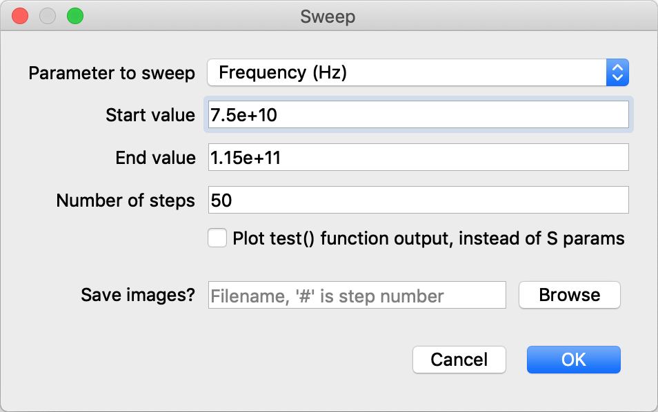
The “parameter to sweep” is one of the parameters defined by the model. The start and end values default to the min and max values of the parameter. The “number of steps” is the number of solves that will be done as the parameter goes from the start to the end value.
If the filename text box is filled in (either by entering a filename there or by selecting the Browse button) then after each solve the model window will be saved to a PNG image. The filename must end in .png and contain a # which will be substituted for the step number.
Once the sweep has completed the sweep tab will show a plot of the results:

Within the plot window, zoom in by left clicking and dragging to select an area of the plot. Zoom out to the previous view by right clicking.
If the “Plot test()” checkbox was not ticked, the plot will show the S-parameters at each port, which is a measurement of the amount of power exiting the port (relative to the excited port).
If the “Plot test()” checkbox was ticked, the plot will show the values returned by the config.test function.
The multi-choice box that defaults to “Magnitude” can be used to select what is plotted, either the magnitude, phase or group delay of the plotted values.
Rama's optimizer adjusts selected parameters to improve the output of the config.optimize function. This can often be much faster than hand tuning parameters to find a desired configuration. For example, optimizing all 5 geometry parameters in the model_ALMA_coupler_Exy.lua model (included with Rama) takes only a second or two.
To use the optimizer, here are the steps:
Define the config.optimize function, referring to the Config table section. The optimizer will adjust parameters to try to make all outputs of the optimize function as close to zero as possible. There are a few tricks to writing this function to achieve better performance:
If you are optimizing multiple things, return multiple values from optimize. For example if you want the returned power from ports 1 and 2 to both be zero, you should return port_power[1], port_power[2]. An alternative single return value is possible, return port_power[1]^2 + port_power[2]^2 and this will have the same optimal point, but by combining both optimization targets into a single return value you are removing information that the optimizer can use to do a better job.
The optimizer tries to push all return values close to zero, so negative return values will be pushed positively toward zero, and positive return values will be pushed negatively toward zero. There is no need to force return values to be positive, e.g. by squaring values.
Complex return values can not be returned directly, return the real and imaginary parts separately.
Where possible limit discontinuities in the optimize function. For example return port_power[1] and return math.abs(port_power[1]) both express the same optimal point, but the discontinuity of the abs function will make that optimization converge more slowly.
Select the parameters to optimize by ticking the checkboxes to the left of the parameter names. A range of checkboxes can be ticked by selecting one and then selecting another with shift pressed. The more parameters are selected, the longer optimization will take. Any parameter can be selected, not just parameters that control the geometry.
Move the selected parameters to their initial values. The optimization will converge to a locally optimal configuration that may be somewhat close to the initial values. Better configurations that are further away may not be explored unless you start with parameter values close to that. So before optimization is attempted you should manually explore how the solution looks across a range of parameter values, and start with parameter values near to where you think a reasonable configuration is.
(Optionally) select the optimization method with the “Solve / Select optimizer” menu. The options are:
Levenberg-Marquardt: a gradient based technique that works for most problems. This is a fast optimization technique, but it is local, in the sense that it will find a locally optimal solution that is close to the starting parameters but can leave unexplored better solutions that are further away.
Subspace Dogleg: a gradient based local optimization technique that has similar performance to Levenberg-Marquardt. This can be a better choice for a small number of problems.
Nelder-Mead / Simulated annealing: a hybrid of those two techniques, that first does a global optimization that gradually reduces temperature, then does a downhill only optimization to find the final solution. Selecting this will pop up a dialog box allowing the technique's many parameters to be configured.
Random search: this just randomly tries solutions until the optimization is stopped, whereupon the best solution found so far is used. This is usually not an efficient choice.
Run the optimizer with the “Solve / Start optimization” menu command. The parameters will be adjusted and the field will be solved repeatedly as the optimizer searches for a solution. If the process is taking too long you can select “Solve / Stop sweep or optimization” to abort it. When convergence is achieved a message will be displayed with convergence information.
If you are not happy with the solution, you can always tweak the parameter values and try again, or change the set of parameters that is optimized. It will often be necessary to tweak the optimize function to achieve satisfactory results, after observing the results of a few optimizations.
Often config.frequency is a single number, and each field solution is for that particular frequency. However config.frequency can be an array of numbers to solve for multiple frequencies simultaneously. There are two reasons to want this: wideband optimization and pulse visualization.
If the current model has multiple frequencies then the “Frequency” spinner and slider at the top of the model window will be enabled, letting you select which of the solutions is currently displayed.
Many functions in Rama will apply only to the currently displayed solution: for example, sweeps and the antenna plot.
The “S Params” window plots the S parameters across all the frequencies in the model. However if an S parameter plot is all that is desired it is generally simpler to use the Sweep command to sweep a frequency parameter. Computing multiple frequencies can be slower per update, as the model needs to be solved multiple times.
If config.frequency is an array of more than one frequency, the config.optimize function can query the solution for each frequency independently. Optimizing the model for multiple frequencies simultaneously can result in models with wider bandwidth. For example, when config.optimize returns the worst return loss over all frequencies, that tends to minimize the return loss over the entire bandwidth.
The port_power and port_phase arguments to config.optimize are just for the currently displayed solution. To query other solutions use the field.Select(n) function to select the frequency that subsequent field functions will apply to. The field.Ports() function will return the arrays of port_power and port_phase that correspond to the currently selected solution.
If the “Wideband pulse” checkbox is ticked and the model has solutions for multiple frequencies then the displayed field is all solutions added together. This results in a pulse, i.e. a short time burst of energy. In many situations it can be instructive to look at how a pulse propagates through the system. The width and duration of the pulse is controlled by the total bandwidth and number of values in config.frequency.
When animating the pulse each solution is advanced in phase by the appropriate amount so the pulse stays coherent. Unlike the single frequency solution, the displayed field does not repeat for every turn of the time dial. The “Set animation time to 0” command can be used to reset the pulse to its starting state.
There is one subtlety to consider when displaying pulses. The weight given to the solution for each frequency can be controlled to minimize the side lobes of the pulse. This is controlled by config.wideband_window, which selects a window function that provides the weights.
When config.type is TE or TM the TE or TM waveguide modes are computed. The number of modes computed is given by config.max_modes. For each mode the cutoff frequency is displayed. The display selection box allows various components of the E and H fields to be displayed.
When the cutoff frequencies of two modes are very close to each other (or identical) the mode fields recovered will be some linear superposition of whatever you think the “official” modes should look like. E.g. for TM modes in a rectangle with 2:1 aspect ratio, modes 4 and 5 will have this issue. The best that the mode solver can do is find an orthogonal subspace for all modes with the same cutoff frequency.
Ports are line segments. Multiple co-linear ports with co-linear regular boundary segments in between are not supported - they will be merged into a single segment and the distinction between the ports will be lost. This happens because of a limitation in the Clipper library, that we should fix at some point.
Ports in Ez and Exy cavities are intended to support the \(TE_{10}\) mode. For this to work, the port width for Ez or the cavity depth for Exy should be large enough to operate above the cutoff frequency of the waveguide. If the port is too wide, other modes will be possible but only the \(TE_{10}\) mode will be excited or absorbed. The waveguide should be constant width after the port, for a significant fraction of a wavelength, to ensure that the \(TE_{10}\) mode becomes established so that the simulation is physically meaningful for excited or absorbed waves.
To help deal with geometrical tolerancing issues within Rama, shape coordinates have a limited resolution. There are effectively 32 bits to the left and right of the decimal point. This quantizes coordinates to \(2.3\times10^{-10}\) and gives us a maximum coordinate of \(\pm 2.1\times10^9\). This is generally not a problem: for config.unit set to meters, the quantization size is on the order of the atomic spacing in a crystal lattice. This does mean however that you should chose config.unit appropriately for your problem. For example, don't create a circle the diameter of the Earth in microns, because that's \(1.3\times 10^{13}\). Use miles or kilometers instead.
Here are things that Rama does not yet model. Correct modeling of these things may be implemented later, if there is need.
Painting of dielectrics does not work in Exy cavities with finite depth. Areas can be painted, and this will affect the solution, but the solution will not satisfy Maxwell's equations and will not necessarily be physically meaningful. Since this situation results in a 3D field with complex structure, this limitation is not likely to be fixed.
Painting of constant dielectric areas works in Ez cavities and Exy cavities with infinite depth, but painting of dielectric fields does not work in Exy cavities with infinite depth. This limitation will be fixed once we add the dielectric term \((\nabla \epsilon/\epsilon)\times(\nabla\times H)\) to the Helmholtz equation for such fields.
Dielectric painting does not work in TE and TM cavities.
Some ports on areas with non-default \(\epsilon\) or \(\sigma\) are not well matched. This currently happens when
The \(\epsilon\) or \(\sigma\) values have imaginary components, meaning there is attenuation or gain in the material.
Ez models have non-default \(\sigma\) values.
Exy models have non-default \(\sigma\) values and don't have a principle axis of the anisotropy aligned with the port.
Ports that are not well matched do not deliver or absorb energy with perfect efficiency. The effect is most noticeable at output ports where there is some reflected wave. The S parameters computed at poorly matched ports will not be correct.
This is a random selection of documentation about the internals of Rama.
See the instructions on github.
For optimization we need to compute derivatives of the config.optimize function with respect to the parameters. Since config.optimize has multiple return values and there are multiple parameters we are actually computing a jacobian matrix. Computing the jacobian numerically is easy enough, but highly inaccurate for two reasons. First there is the classic problem of choosing the step size \(h\) in \(f'(x) \approx f(x+h)/h\) without introducing either truncation or floating point errors. Second, the more serious problem is that the current mesh generator is not stable so even small changes in boundary geometry can cause completely different meshes to be generated. This means that the field solution (and therefore the objective function) is a little noisy. That noise forces us to use large \(h\), making the jacobian untrustworthy. A bad jacobian will frustrate the ability of e.g. a Levenberg-Marquardt optimizer to reach a good solution.
A much better approach is to compute a correct jacobian, either analytically or using automatic differentiation. In fact we must use both approaches together, as the Lua script contains a user defined function for which we can not figure out analytic jacobians, and a large \(Ax=b\) solve would be slowed down too much if each matrix element was subject to automatic differentiation.
Let's look at the complete chain of dependencies between the parameters \(p\) and the config.optimize output. We use the chain rule to figure out \(d/dp\) at each stage. The dependency chain is:
Start with the parameter vector \(p\).
\(p \rightarrow\) Lua script engine \(\rightarrow S\) (the shape of the computational domain) and the ScriptConfig. We introduce the numerical type JetNum (based on ceres::Jet), which does automatic differentiation. The Lua interpreter is modified to accept JetNum as its lua_Number, meaning that derivatives with respect to parameters can be carried through all numeric quantities in user scripts. All point coordinates in shapes use JetNum, so we automatically have \(dS/dp\).
The main issue with this scheme is the Clipper library, which converts all continuous quantities into integers for its own robustness reasons, so we can not simply replace those integers with JetNum. However each Clipper integer coordinate has an associated Z value, which we modify to contain the required derivatives. The Z derivatives for new vertices introduced by Clipper are computed correctly by the Clipper ZFillCallback.
For simplicity below we enforce that ScriptConfig should not depend on the parameters. This restriction can be relaxed later.
\(dS/dp \rightarrow\) Mesher \(\rightarrow dM/dp\), where \(M\) is the mesh. We must ignore the mesh length and refinement settings in ScriptConfig because they would substantially alter the mesh, and the stability of our method depends on the fact that the mesh remains unaltered. Therefore we enforce that ScriptConfig should not depend on the parameters. The continuous values in the mesh are the vertex positions and triangle material values (e.g. \(\epsilon\)). The other mesh values are triangle connectivity and port settings, discrete values which are assumed not to be affected by small changes in the parameters. For simplicity below we enforce that material settings can not depend on parameters.
To compute \(dM/dp\) we associate boundary triangle edges to lines in \(dS/dp\), then linearly interpolate from \(dS/dp\). We assume that as parameters changes only boundary triangles are affected, i.e. geometry changes are not propagated into interior triangles.
\(dM/dp \rightarrow\) System matrix creator \(\rightarrow dA/dp, db/dp\). This is done with automatic differentiation by using JetNum and JetComplex.
\(dA/dp, db/dp \rightarrow\) Linear solver \(\rightarrow dx/dp\). Given a solution to a linear problem \(A \: x = b\) and a scalar parameter \(p\), we want to compute \(dx/dp\) from \(dA/dp\) and \(db/dp\), without expensive refactoring of \(A\)-sized matrices. From the Matrix Cookbook we have
\[\begin{align} {\del A^{-1} \by \del p} &= -A^{-1} \: {\del A \by \del p} \: A^{-1} \end{align}\]From which we get
\[\begin{align} x &= A^{-1} \: b \\ {\del x \by \del p} &= {\del A^{-1} \by \del p} \: b + A^{-1} \: {\del b \by \del p} \\ &= -A^{-1} \: {\del A \by \del p} \: A^{-1} \: b + A^{-1} \: {\del b \by \del p} \\ &= A^{-1} \left( -{\del A \by \del p} \: x + {\del b \by \del p} \right) \end{align}\]The cost of this is one multiplication by \(\del A / \del p\) (which might be cheap if it is sparse) and one solve with the already factored \(A^{-1}\).
\(dx/dp \rightarrow\) Compute port powers \(\rightarrow P\), where \(P\) are the port powers and phase angles. This is done with JetNum.
\(P \rightarrow\) output of the config.optimize function. This is done with JetNum within Lua.
Each JetNum contains the derivative with respect to just one parameter, so the above steps have to be done once per parameter. The JetNum could contain more derivatives but that would slow down the Lua interpreter, and we spend most of the time doing the matrix solves anyway.
Rama is open source software that anyone is free to use and modify. It is licensed to you under the terms of the GNU General Public License, version 3 (or GPLv3).
Rama is built upon many other open source software libraries, that each have their own licenses. Those other licenses are linked in the Rama COPYING file. The licenses vary widely in what they permit, but the most restrictive of them are also GPLv3.
For details of Rama's own license, please see the Rama COPYING file. However, to summarise:
Anyone can use this software, free of charge. That includes private, educational, and commercial use.
Anyone can copy, modify and distribute this software.
If you modify this software, your modifications must also be licensed under GPLv3.
If you distribute this software, those who receive it must inherit these same rights and responsibilities.
This software is provided without any warranty.
The authors of this software can not be held liable for any damages inflicted by the software.
All copyrights are held by the respective authors.
Here is what is added in each new version.
v0.36
Added the “coincident vertex rule” for shape booleans.
Added the shape s.material property.
Added the shape vertex kind0,kind1,dist0,dist1 properties
Added util.Dump().
Fixed a bug that sometimes caused ports to be defective when added after dielectric painting (consistent EdgeInfo on coincident vertices).
Added s:HasPorts().
Warn about NaN derivatives in port callback values.
Fix field.Complex() dummy evaluation.
Warn about nonfinite or non number return values in config.optimize().
Fix s:Grow to work with two point polylines.
Documented the util table.
Added utilities for modeling the loss from good conductors (PaintMetal and PortMetal).
v0.37
Support for ES cavities, for electrostatics.
Added the conj field to complex numbers.
Added LoadSTL functions to shape and util.
Fix crashing bug for necked zero area polygons (in SplitPolygonsAtNecks).
It's now an error if infinity is passed as a numerical argument to a shape function.
Slightly improved display scaling of vector fields.
Added examples: capacitor_electrostatics.lua, photonic_nanojet.lua
Fixed waveguide mode vector scaling.
Make available the time related functions in the os library.
Fix bug that caused sweep integer parameter values to sometimes be slightly non integer.
Warn about parameter creation that depends on other parameters.
Fix math.random() on windows.
Various minor stability improvement.
v0.38
Added the 3D viewing mode.
Improved Windows track pad support.
FilletVertex can now construct fillets that are tangent to just one edge of the vertex if it is impossible to make it tangent to both edges.
Fix a bug in Clean where duplicate points were not removed.
Added dxf_arc_dist and dxf_arc_angle to allow DXF files to contain arcs.
Added Nelder-Mead and simulated annealing optimization techniques.
Upgrade to Lua 5.4.1.
Changed the return value of ChamferVertex.
Default directory for dofile and saves is the script directory.
Move MakeMachinable to the util table.
Parameter{} called again with identical arguments returns the same value as last time.
Added util.include.
Added util.script_filename.
Added util.VertexOnPort.
Added the defaults argument to Parameter.
Added vector functions: length, dot, cross, vec.New, vec.Normalize.
Behavior change in FilletVertex, and new information returned.
Add shape concatenation operator.
s:AddPoint can now accept the table returned by s[i].
Added the shape s.self_intersection property.
Expanded arguments to s:Clean().
Fixed the documentation for the s.bounds value.